44 add labels to bar chart excel
› gantt-chart › how-to-makeExcel Gantt Chart Tutorial + Free Template + Export to PPT To create a Gantt chart in Excel that you can use as a template in the future, you need to do the following: List your project data into a table with the following columns: Task description, Start date, End date, Duration. Add a Stacked Bar Chart to your Excel spreadsheet using the Chart menu under the Insert tab. › how-to-create-bar-chart-withHow to Create a Bar Chart With Labels Above Bars in Excel In the chart, right-click the Series "Dummy" Data Labels and then, on the short-cut menu, click Format Data Labels. 15. In the Format Data Labels pane, under Label Options selected, set the Label Position to Inside End. 16. Next, while the labels are still selected, click on Text Options, and then click on the Textbox icon. 17.
Add data labels and callouts to charts in Excel 365 - EasyTweaks.com Step #1: After generating the chart in Excel, right-click anywhere within the chart and select Add labels . Note that you can also select the very handy option of Adding data Callouts.

Add labels to bar chart excel
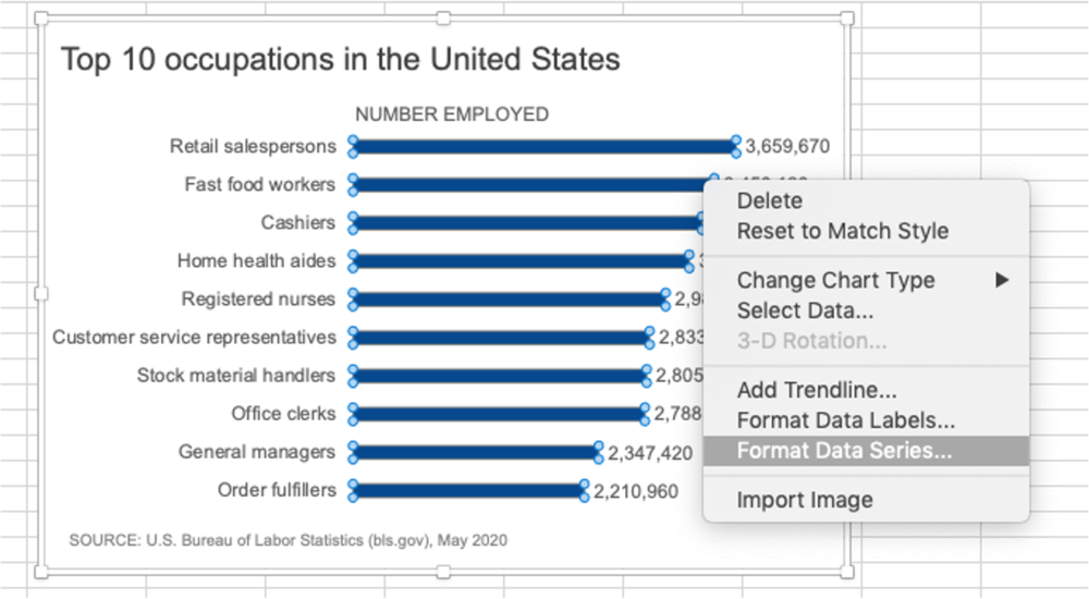
How to place labels underneath bar chart - Microsoft Community Answer jpgpinto Replied on February 20, 2012 The names are appearing below the chart axis, that is on value 0.0%. They are on the correct place. If you want them to appear at the bottom of your chart, just select the axis and on the "Format axis" dialog box, on the "Axis options" tab, on the "Axis labels:" option, select "Low". jpgpinto How to add or move data labels in Excel chart? - ExtendOffice In Excel 2013 or 2016. 1. Click the chart to show the Chart Elements button . 2. Then click the Chart Elements, and check Data Labels, then you can click the arrow to choose an option about the data labels in the sub menu. See screenshot: In Excel 2010 or 2007. 1. click on the chart to show the Layout tab in the Chart Tools group. See ... › charts › variance-clusteredActual vs Budget or Target Chart in Excel - Variance on ... Aug 19, 2013 · This gives you the value for plotting the base column/bar of the stacked chart. The bar in the chart is actually hidden behind the clustered chart. _ Positive Variance – The variance is calculated as the variance between series 1 and series 2 (actual and budget). This is displayed as a positive result.
Add labels to bar chart excel. Text Labels on a Horizontal Bar Chart in Excel - Peltier Tech On the Excel 2007 Chart Tools > Layout tab, click Axes, then Secondary Horizontal Axis, then Show Left to Right Axis. Now the chart has four axes. We want the Rating labels at the bottom of the chart, and we'll place the numerical axis at the top before we hide it. In turn, select the left and right vertical axes. Add Labels ON Your Bars - Evergreen Data Then insert a basic bar chart. Right-click on one of the Label bars and select Format Data Series. Change the fill color to No Fill. Then right-click on one of those bars again and select Add Data Labels. This will add 35% to the end of every Label bar you just turned No Fill. Right-click on those labels and select Format Data Labels. How to Add Category Labels AND Data labels to the Same Bar Chart in ... #excel #dataviz #barchartHere's a great trick for when you need your bar chart's category label appear on one side of the bar and your data label to appear o... Excel charts: add title, customize chart axis, legend and data labels Click anywhere within your Excel chart, then click the Chart Elements button and check the Axis Titles box. If you want to display the title only for one axis, either horizontal or vertical, click the arrow next to Axis Titles and clear one of the boxes: Click the axis title box on the chart, and type the text.
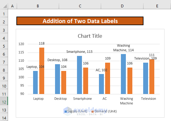
How to Add Axis Labels in Excel Charts - Step-by-Step (2022) - Spreadsheeto How to add axis titles 1. Left-click the Excel chart. 2. Click the plus button in the upper right corner of the chart. 3. Click Axis Titles to put a checkmark in the axis title checkbox. This will display axis titles. 4. Click the added axis title text box to write your axis label. How to Insert Axis Labels In An Excel Chart | Excelchat We will go to Chart Design and select Add Chart Element Figure 6 - Insert axis labels in Excel In the drop-down menu, we will click on Axis Titles, and subsequently, select Primary vertical Figure 7 - Edit vertical axis labels in Excel Now, we can enter the name we want for the primary vertical axis label. Adding rich data labels to charts in Excel 2013 To add a data label in a shape, select the data point of interest, then right-click it to pull up the context menu. Click Add Data Label, then click Add Data Callout . The result is that your data label will appear in a graphical callout. In this case, the category Thr for the particular data label is automatically added to the callout too. How to Add Two Data Labels in Excel Chart (with Easy Steps) Table of Contents hide. Download Practice Workbook. 4 Quick Steps to Add Two Data Labels in Excel Chart. Step 1: Create a Chart to Represent Data. Step 2: Add 1st Data Label in Excel Chart. Step 3: Apply 2nd Data Label in Excel Chart. Step 4: Format Data Labels to Show Two Data Labels. Things to Remember.
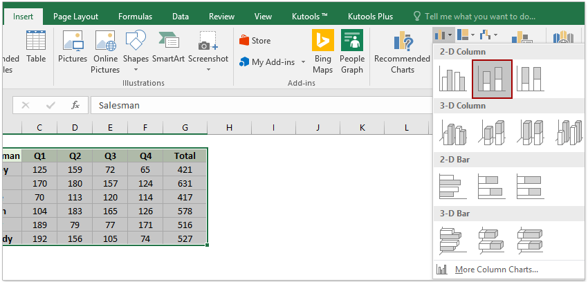
› add-vertical-line-excel-chartAdd vertical line to Excel chart: scatter plot, bar and line ... Oct 20, 2022 · To create a vertical line in your Excel chart, please follow these steps: Select your data and make a bar chart (Insert tab > Charts group > Insert Column or Bar chart > 2-D Bar). In some empty cells, set up the data for the vertical line like shown below. Add or remove data labels in a chart - support.microsoft.com Add data labels to a chart Click the data series or chart. To label one data point, after clicking the series, click that data point. In the upper right corner, next to the chart, click Add Chart Element > Data Labels. To change the location, click the arrow, and choose an option. How to add data labels to a Column (Vertical Bar) Graph in ... - YouTube Get to know about easy steps to add data labels to a Column (Vertical Bar) Graph in Microsoft® Excel 2010 by watching this video.Content in this video is pro... How to Make a Bar Chart in Microsoft Excel - How-To Geek Adding and Editing Axis Labels To add axis labels to your bar chart, select your chart and click the green "Chart Elements" icon (the "+" icon). From the "Chart Elements" menu, enable the "Axis Titles" checkbox. Axis labels should appear for both the x axis (at the bottom) and the y axis (on the left). These will appear as text boxes.
Dynamically Label Excel Chart Series Lines • My Online ...
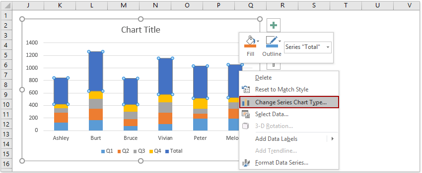
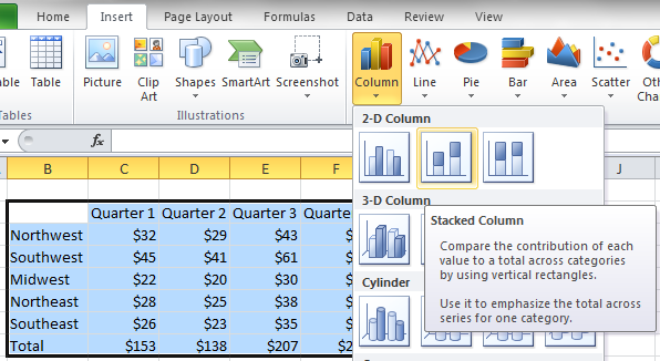
How to add total labels to stacked column chart in Excel? - ExtendOffice Add total labels to stacked column chart in Excel Supposing you have the following table data. 1. Firstly, you can create a stacked column chart by selecting the data that you want to create a chart, and clicking Insert > Column, under 2-D Column to choose the stacked column. See screenshots: And now a stacked column chart has been built. 2.
How to make a bar graph in Excel
spreadsheetplanet.com › bar-of-pie-chart-excelHow to Create Bar of Pie Chart in Excel? Step-by-Step Excel lets us add our own customizations to the Bar of Pie chart. For example, it lets us specify how we want the portions to get split between the pie and the stacked bar. It also lets us specify whether we want to display data labels, what data labels we want to be displayed as well as what formatting and styling we want to apply to the labels.
Labeling a Stacked Column Chart in Excel - PolicyViz
› excel › how-to-add-total-dataHow to Add Total Data Labels to the Excel Stacked Bar Chart Apr 03, 2013 · For stacked bar charts, Excel 2010 allows you to add data labels only to the individual components of the stacked bar chart. The basic chart function does not allow you to add a total data label that accounts for the sum of the individual components. Fortunately, creating these labels manually is a fairly simply process.

excel - How to show series-Legend label name in data labels ...
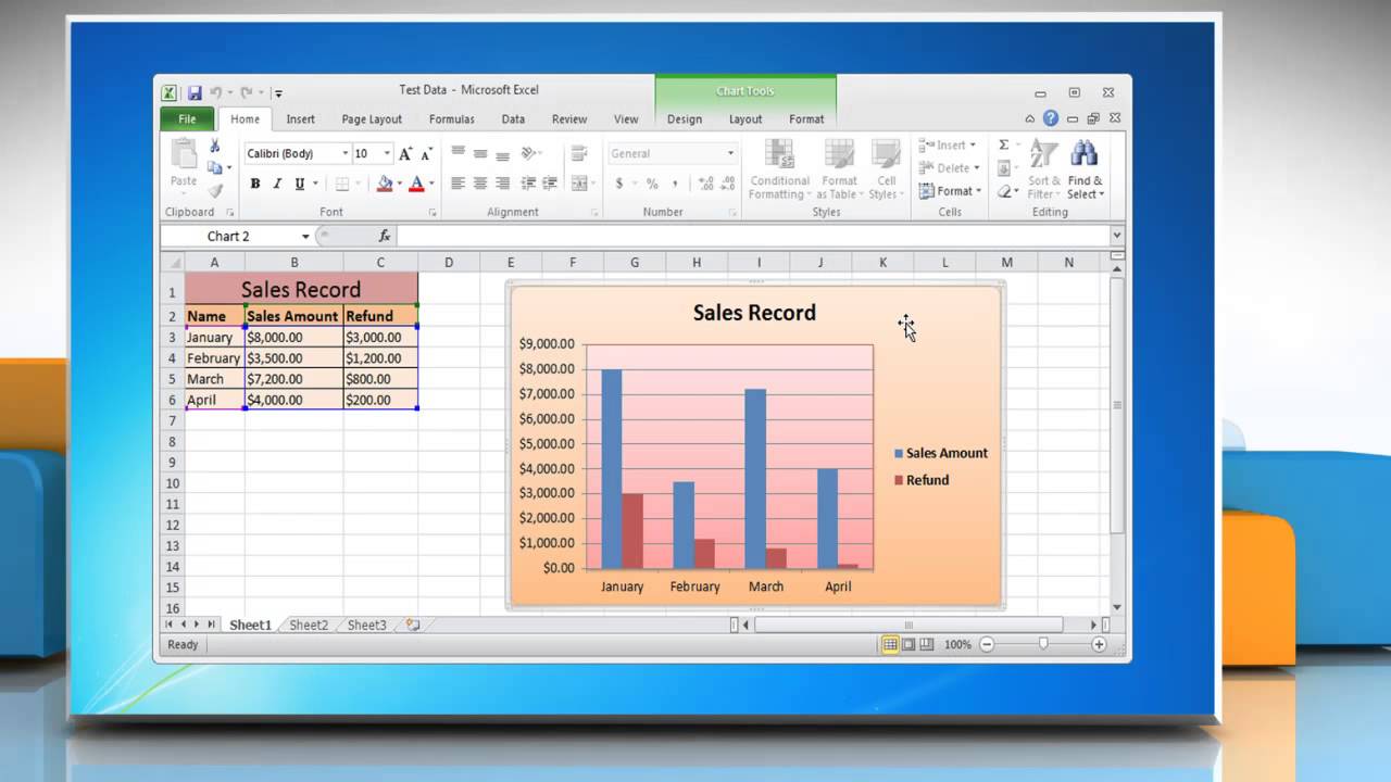
Bar Chart in Excel (Examples) | How to Create Bar Chart in Excel? - EDUCBA Step 9: To add Labels to the bar Right click on bar > Add Data Labels; click on it. Data Label is added to each bar. Similarly, you can choose different colors for each bar separately. I have chosen different colors, and my chart is looking like this. Example #2 There are multiple bar graphs available.
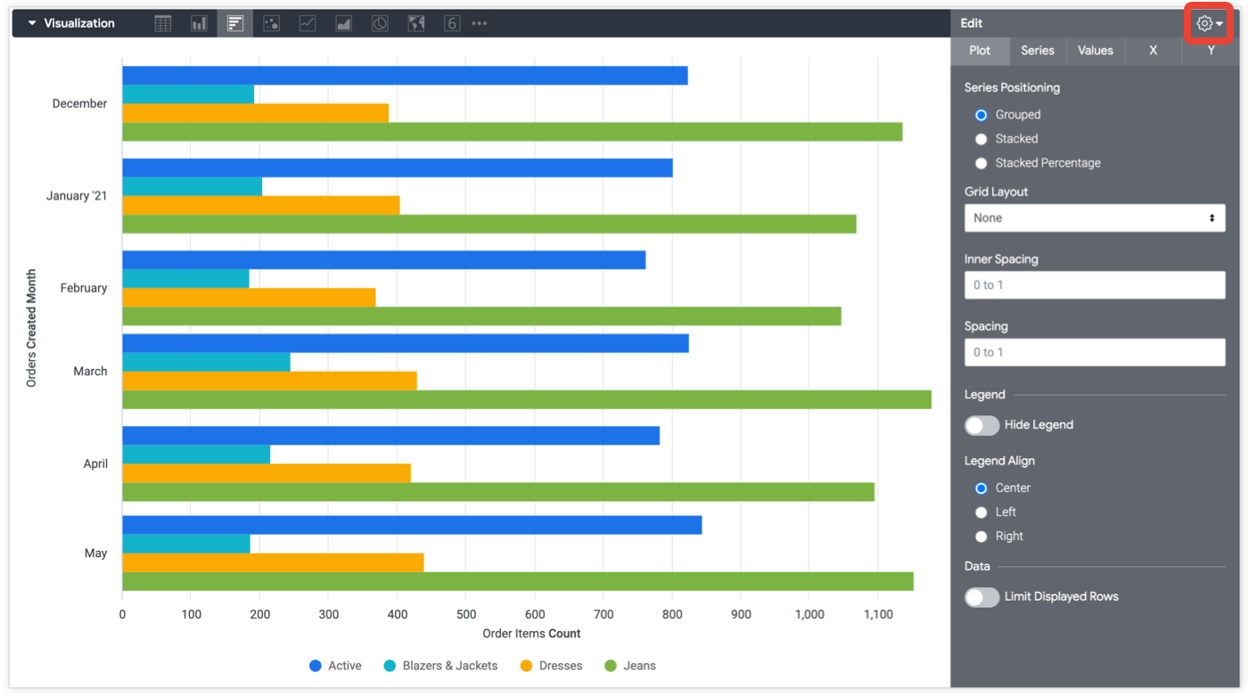
Bar chart options | Looker | Google Cloud
Multiple Data Labels on bar chart? - Excel Help Forum Select A1:D4 and insert a bar chart. Select 2 series and delete it. Select 2 series, % diff base line, and move to secondary axis. Adjust series 2 data references, Value from B2:D2. Category labels from B4:D4. Apply data labels to series 2 outside end. select outside end data labels and change from Values to Category Name.

Add Labels ON Your Bars
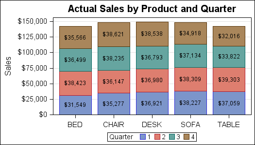
How to Add Total Values to Stacked Bar Chart in Excel Step 4: Add Total Values. Next, right click on the yellow line and click Add Data Labels. Next, double click on any of the labels. In the new panel that appears, check the button next to Above for the Label Position: Next, double click on the yellow line in the chart. In the new panel that appears, check the button next to No line:

How to add total labels to stacked column chart in Excel?
How to Add Data Labels to an Excel 2010 Chart - dummies Use the following steps to add data labels to series in a chart: Click anywhere on the chart that you want to modify. On the Chart Tools Layout tab, click the Data Labels button in the Labels group. None: The default choice; it means you don't want to display data labels. Center to position the data labels in the middle of each data point.

Aligning data point labels inside bars | How-To | Data ...
Excel: How to Create a Bubble Chart with Labels - Statology To add labels to the bubble chart, click anywhere on the chart and then click the green plus "+" sign in the top right corner. Then click the arrow next to Data Labels and then click More Options in the dropdown menu: In the panel that appears on the right side of the screen, check the box next to Value From Cells within the Label Options ...

Add Total Values for Stacked Column and Stacked Bar Charts in ...
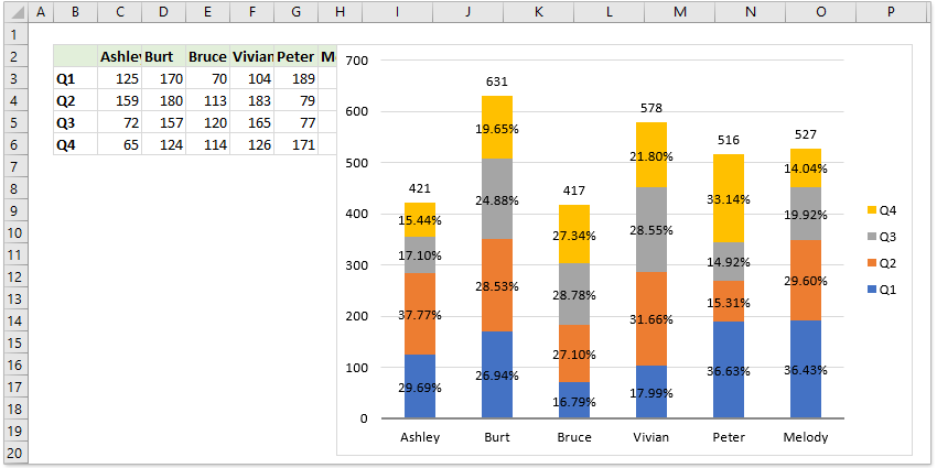
How to Show Percentage in Bar Chart in Excel (3 Handy Methods) - ExcelDemy 📌 Step 02: Insert Stacked Column Chart and Add Labels Secondly, select the dataset and navigate to Insert > Insert Column or Bar Chart > Stacked Column Chart. Similar to the previous method, switch the rows and columns and choose the Years as the x-axis labels. Next, go to Chart Element > Data Labels.
Excel Bar Chart with Vertical Line • My Online Training Hub
Edit titles or data labels in a chart - support.microsoft.com On a chart, click the label that you want to link to a corresponding worksheet cell. On the worksheet, click in the formula bar, and then type an equal sign (=). Select the worksheet cell that contains the data or text that you want to display in your chart. You can also type the reference to the worksheet cell in the formula bar.

How to Add Total Data Labels to the Excel Stacked Bar Chart ...
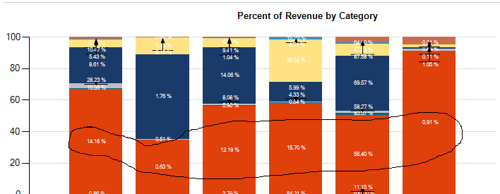
How to Add Percentages to Excel Bar Chart We will select range A1:C8 and go to Insert >> Charts >> 2-D Column >> Stacked Column: Once we do this we will click on our created Chart, then go to Chart Design >> Add Chart Element >> Data Labels >> Inside Base: To lose the colors that we have on points percentage and to lose it in the title we will simply click anywhere on the small orange ...
/simplexct/BlogPic-h7046.jpg)
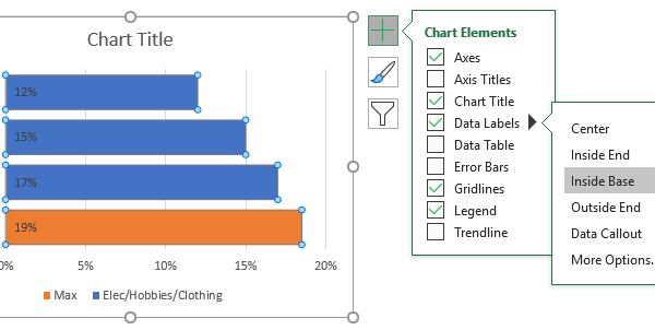
How to Create a Bar Chart With Labels Above Bars in Excel
HOW TO CREATE A BAR CHART WITH LABELS INSIDE BARS IN EXCEL - simplexCT 7. In the chart, right-click the Series "# Footballers" Data Labels and then, on the short-cut menu, click Format Data Labels. 8. In the Format Data Labels pane, under Label Options selected, set the Label Position to Inside End. 9. Next, in the chart, select the Series 2 Data Labels and then set the Label Position to Inside Base.
How to add total labels to stacked column chart in Excel?
› pulse › how-add-total-stackedHow to add a total to a stacked column or bar chart in ... Sep 07, 2017 · The method used to add the totals to the top of each column is to add an extra data series with the totals as the values. Change the graph type of this series to a line graph.

data visualization - How do you put values over a simple bar ...
How can I add custom labels to each bar in a graph? Here are the steps for the picture above: 1) Create Bar Chart from data range of A1:C21. 2) Delete Horizontal Gridlines. 3) Delete Legend. 4) Change Fill Colors for Each Series. 5) Change Vertical Axis to "categories in reverse order" so that the labels are in the right order.
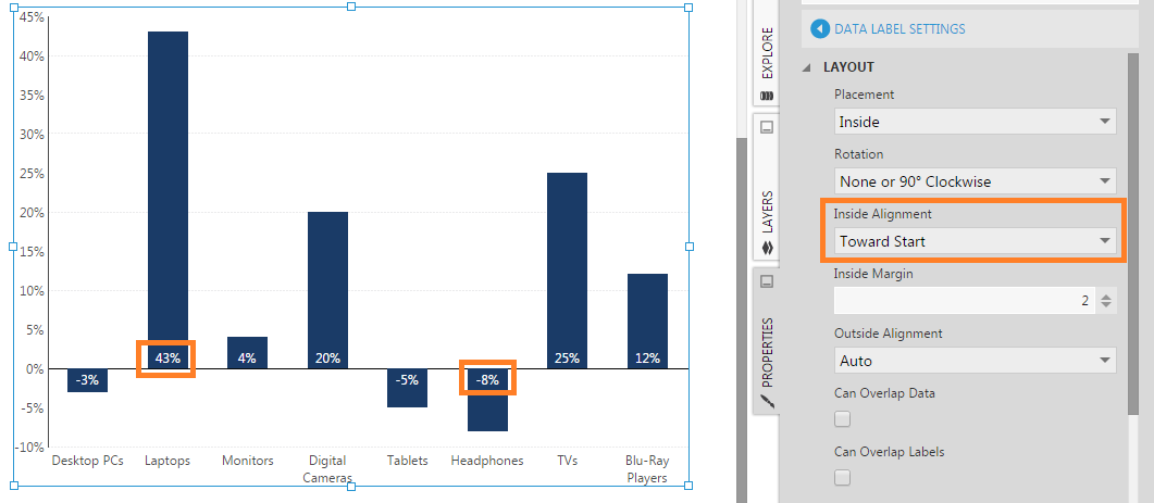
Aligning data point labels inside bars | How-To | Data ...
2 data labels per bar? - Microsoft Community If people want to see patterns in the data and quickly assimilate this without having to compute things, then a simple, uncluttered chart is ideal. So if you are creating a report for a mixed audience, maybe you need both. But adding lots of labels all over your chart is giving nobody the best result.

How to Add Total Data Labels to the Excel Stacked Bar Chart ...
› charts › variance-clusteredActual vs Budget or Target Chart in Excel - Variance on ... Aug 19, 2013 · This gives you the value for plotting the base column/bar of the stacked chart. The bar in the chart is actually hidden behind the clustered chart. _ Positive Variance – The variance is calculated as the variance between series 1 and series 2 (actual and budget). This is displayed as a positive result.
Labeling a Stacked Column Chart in Excel - PolicyViz
How to add or move data labels in Excel chart? - ExtendOffice In Excel 2013 or 2016. 1. Click the chart to show the Chart Elements button . 2. Then click the Chart Elements, and check Data Labels, then you can click the arrow to choose an option about the data labels in the sub menu. See screenshot: In Excel 2010 or 2007. 1. click on the chart to show the Layout tab in the Chart Tools group. See ...
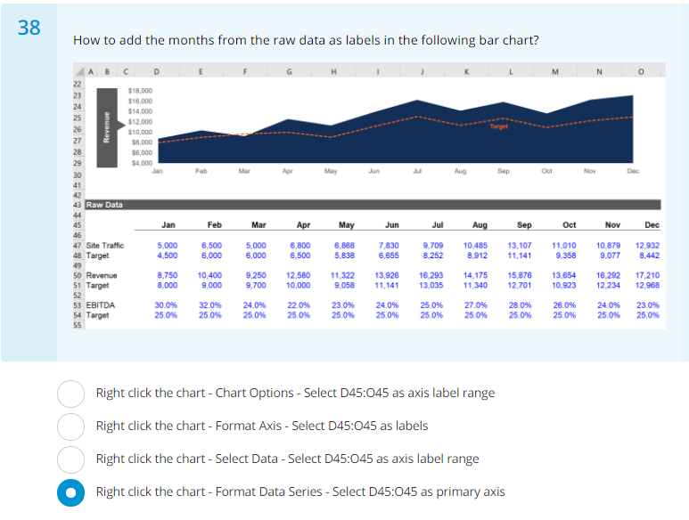
Solved 38 How to add the months from the raw data as labels ...
How to place labels underneath bar chart - Microsoft Community Answer jpgpinto Replied on February 20, 2012 The names are appearing below the chart axis, that is on value 0.0%. They are on the correct place. If you want them to appear at the bottom of your chart, just select the axis and on the "Format axis" dialog box, on the "Axis options" tab, on the "Axis labels:" option, select "Low". jpgpinto
How to format bar charts in Excel — storytelling with data

Add or remove data labels in a chart
Creating Excel Stacked Column Chart Label Leader Lines/Spines ...

Bar Chart Target Markers - Excel University

Add Data Labels for Total to Stacked Columns in #Excel | wmfexcel
How to add data labels to a Column (Vertical Bar) Graph in Microsoft® Excel 2010

How to use data labels in a chart

How to Add and Remove Chart Elements in Excel
How to add total labels to stacked column chart in Excel?
How to add total labels to stacked column chart in Excel?
Percentages as Labels for Stacked Bar Charts | SQL Server ...
Excel Data Labels: How to add totals as labels to a stacked ...
The Data School - Two ways to add labels to the right inside ...

Adding rich data labels to charts in Excel 2013 | Microsoft ...
Aligning data point labels inside bars | How-To | Data ...
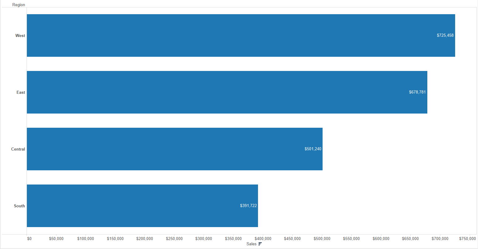
Text Labels on a Horizontal Bar Chart in Excel - Peltier Tech

How to Add Data Labels to an Excel 2010 Chart - dummies

How to Add Two Data Labels in Excel Chart (with Easy Steps ...
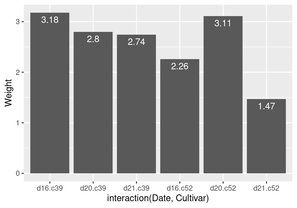
3.9 Adding Labels to a Bar Graph | R Graphics Cookbook, 2nd ...
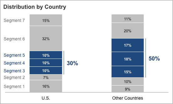
Stacked Bar Chart with Segment Labels - Graphically Speaking

Adding rich data labels to charts in Excel 2013 | Microsoft ...
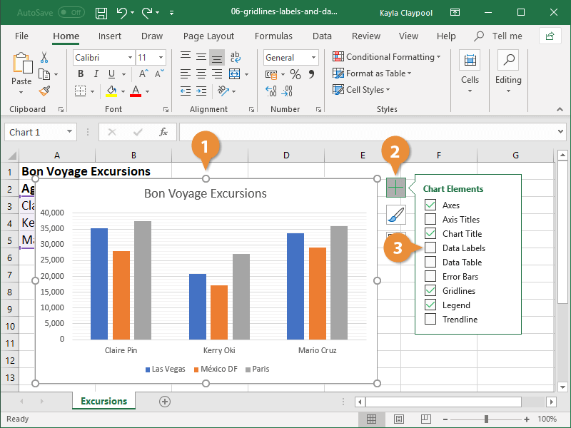
How to Add Axis Labels to a Chart in Excel | CustomGuide
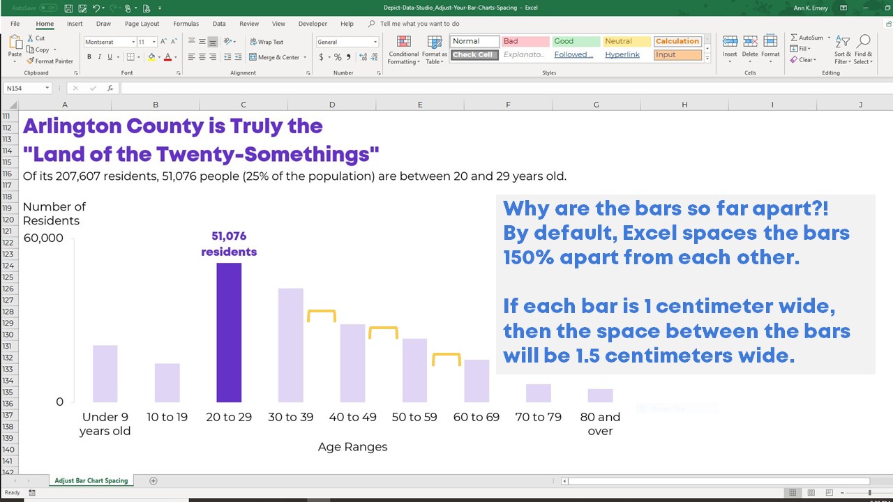
How to Adjust Your Bar Chart's Spacing in Microsoft Excel ...
How to Add Totals to Stacked Charts for Readability - Excel ...

Total of chart series – Excel kitchenette
How to Add Two Data Labels in Excel Chart (with Easy Steps ...
Post a Comment for "44 add labels to bar chart excel"