43 how to add data labels to a 3d pie chart in excel

How To Make a Pie Chart in Excel (With Tips) | Indeed.com Select the information and create the chart. Using your mouse, click on the cell in the top left corner and drag until you've highlighted each cell with a category or number in it. Next, click "Insert" at the top left of your window. Depending on the version, you might select "Insert pie or doughnut chart" or an icon of a pie chart, which opens ... › pie-chart-makerFree Pie Chart Maker - Make Your Own Pie Chart | Visme To use the pie chart maker, click on the data icon in the menu on the left. Enter the Graph Engine by clicking the icon of two charts. Choose the pie chart option and add your data to the pie chart creator, either by hand or by importing an Excel or Google sheet.

How to display leader lines in pie chart in Excel? - ExtendOffice To display leader lines in pie chart, you just need to check an option then drag the labels out. 1. Click at the chart, and right click to select Format Data Labels from context menu. 2. In the popping Format Data Labels dialog/pane, check Show Leader Lines in the Label Options section. See screenshot: 3.

How to add data labels to a 3d pie chart in excel

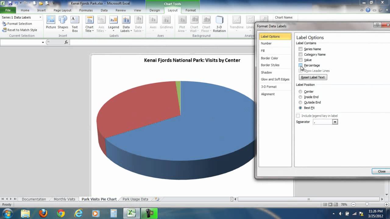
How to Make a Pie Chart in Excel & Add Rich Data Labels to The Chart! 7) With the data point still selected, go to Chart Tools>Format>Shape Styles and click on the drop-down arrow next to Shape Effects and select Shadow and choose Inner Shadow>Inside Diagonal Top Left. 8) With the one data point still selected, right-click this data point, and select Add Data Label>Add Data Callout as shown below. How to Make a Pie Chart in Excel - WinBuzzer We show you how to create a Pie Chart in Excel, explode it, and customize its colors, labels, and positioning. By. Ryan Maskell - April 5, 2022 6:13 pm CEST ... Excel 3-D Pie charts - Microsoft Excel 2013 - OfficeToolTips 2. On the Insert tab, in the Charts group, choose the Pie button: Choose 3-D Pie . 3. Right-click in the chart area. In the popup menu select Add Data Labels and then click Add Data Labels : 4. Click in one of labels to select all of them, then right-click and select the Format Data Labels... in the popup menu: 5.

How to add data labels to a 3d pie chart in excel. 2D & 3D Pie Chart in Excel - Tech Funda To plot the Target data on the chart, select 'Target' series radio button and click 'Apply' button. Similarly, to hide any of the months plots on the chart de-select he checkbox and click on Apply. 3-D Pie Chart To create 3-D Pie chart, select 3-D Pie chart from Insert Chart dropdown (Look at the 1 st picture above). How to Create a Pie Chart in Excel - Smartsheet Enter data into Excel with the desired numerical values at the end of the list. Create a Pie of Pie chart. Double-click the primary chart to open the Format Data Series window. Click Options and adjust the value for Second plot contains the last to match the number of categories you want in the "other" category. How to show percentage in pie chart in Excel? - ExtendOffice Please do as follows to create a pie chart and show percentage in the pie slices. 1. Select the data you will create a pie chart based on, click Insert > I nsert Pie or Doughnut Chart > Pie. See screenshot: 2. Then a pie chart is created. Right click the pie chart and select Add Data Labels from the context menu. 3. adding decimal places to percentages in pie charts Hello DV_1956. I am V. Arya, Independent Advisor, to work with you on this issue. Right click on your % label - Format Data labels. Beneath Number choose percentage as category. Report abuse. 41 people found this reply helpful. ·. Was this reply helpful?

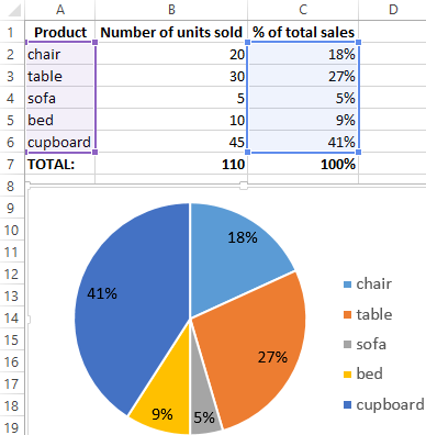
Pie Chart in Excel | How to Create Pie Chart - EDUCBA In this way, we can present our data in a PIE CHART makes the chart easily readable. Example #2 – 3D Pie Chart in Excel. Now we have seen how to create a 2-D Pie chart. We can create a 3-D version of it as well. For this example, I have taken sales data as an example. I have a sale person name and their respective revenue data. How to Add Data Labels to an Excel 2010 Chart - dummies Use the following steps to add data labels to series in a chart: Click anywhere on the chart that you want to modify. On the Chart Tools Layout tab, click the Data Labels button in the Labels group. None: The default choice; it means you don't want to display data labels. Center to position the data labels in the middle of each data point. Free Pie Chart Maker - Make Your Own Pie Chart | Visme Create pie charts with our online pie chart maker. Import Excel data or sync to live data with our pie chart maker. Add several data points, data labels to each slice of pie. Chosen by brands large and small . Our pie chart maker is used by over 14,209,854 marketers, communicators, executives and educators from over 120 countries that include: EASY TO EDIT Pie Chart Templates. Make your data ... › how-to-show-percentage-inHow to Show Percentage in Pie Chart in Excel? - GeeksforGeeks Jun 29, 2021 · Select a 2-D pie chart from the drop-down. A pie chart will be built. Select -> Insert -> Doughnut or Pie Chart -> 2-D Pie. Initially, the pie chart will not have any data labels in it. To add data labels, select the chart and then click on the “+” button in the top right corner of the pie chart and check the Data Labels button.

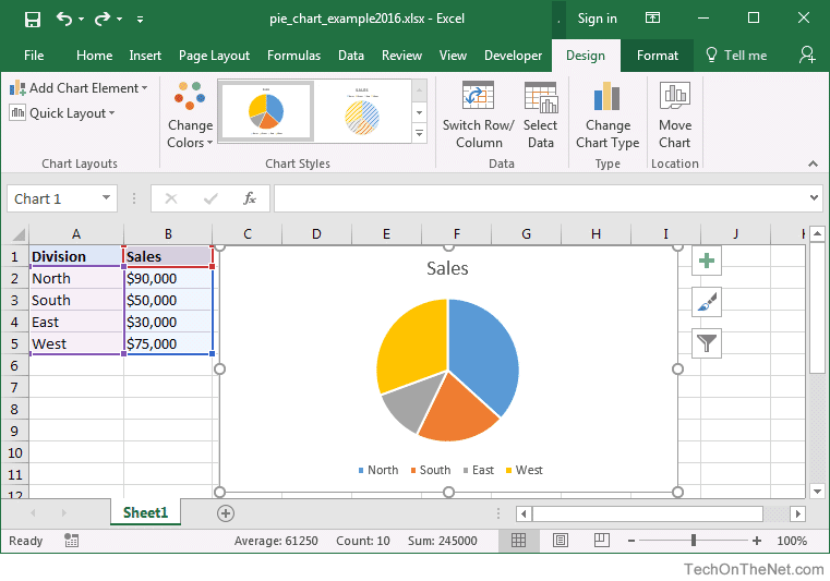
How to Create and Format a Pie Chart in Excel - Lifewire To add data labels to a pie chart: Select the plot area of the pie chart. Right-click the chart. Select Add Data Labels . Select Add Data Labels. In this example, the sales for each cookie is added to the slices of the pie chart. Change Colors Microsoft Excel Tutorials: Add Data Labels to a Pie Chart To add the numbers from our E column (the viewing figures), left click on the pie chart itself to select it: The chart is selected when you can see all those blue circles surrounding it. Now right click the chart. You should get the following menu: From the menu, select Add Data Labels. New data labels will then appear on your chart: 3D Plot in Excel | How to Plot 3D Graphs in Excel? - EDUCBA For that, select the data and go to the Insert menu; under the Charts section, select Line or Area Chart as shown below. After that, we will get the drop-down list of Line graphs as shown below. From there, select the 3D Line chart. After clicking on it, we will get the 3D Line graph plot as shown below. › plot-a-pie-chart-in-pythonPlot a pie chart in Python using Matplotlib - GeeksforGeeks Nov 30, 2021 · Creating Pie Chart. Matplotlib API has pie() function in its pyplot module which create a pie chart representing the data in an array. Syntax: matplotlib.pyplot.pie(data, explode=None, labels=None, colors=None, autopct=None, shadow=False) Parameters: data represents the array of data values to be plotted, the fractional area of each slice is ...

How to Make a Pie Chart in Microsoft Excel 2010

PIE CHART in R with pie() function [WITH SEVERAL EXAMPLES] An alternative to display percentages on the pie chart is to use the PieChart function of the lessR package, that shows the percentages in the middle of the slices.However, the input of this function has to be a categorical variable (or numeric, if each different value represents a category, as in the example) of a data frame, instead of a numeric vector.

3D Doughnut Chart for KPI Metrics - PK: An Excel Expert

Edit titles or data labels in a chart - support.microsoft.com On a chart, click one time or two times on the data label that you want to link to a corresponding worksheet cell. The first click selects the data labels for the whole data series, and the second click selects the individual data label. Right-click the data label, and then click Format Data Label or Format Data Labels.

Excel charts: Mastering pie charts, bar charts and more | PCWorld

Pie Chart In Excel | Microsoft Excel Tips | Excel Tutorial | Free Excel ... Action starts with the selection of data. First prepare a table with data. Then go to the Insert tab in the ribbon Excel. Find and select the Charts section -> Pie. You will insert a pie chart. The question is which one to choose. Pie Chart will look like this: This one is the most basic one. I like it and would choose it for sure. 3D Pie Chart

Add and take the percent from number in Excel with the examples

Create Pie Chart In Excel - PieProNation.com Show percentage in pie chart in Excel. Please do as follows to create a pie chart and show percentage in the pie slices. 1. Select the data you will create a pie chart based on, click Insert> Insert Pie or Doughnut Chart> Pie. See screenshot: 2. Then a pie chart is created. Right click the pie chart and select Add Data Labels from the context ...

How to Create Excel Pie Charts & Add Rich Data Labels to The Chart!

Tips for turning your Excel data into PowerPoint charts 21/08/2012 · Instead, it’s a chart that shows only the data necessary to make the desired point clear – no less, no more. Too much data (sometimes called “data dump”) will overwhelm your audience, blunting your message. Limit the Data. Instead of creating a chart from data in an entire Excel spreadsheet, first edit your spreadsheet. One way to do ...

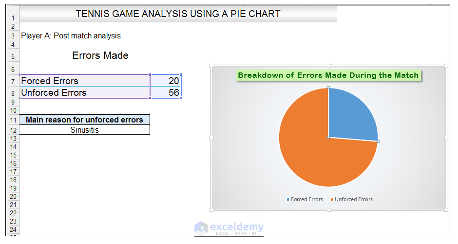
Inserting % and Actual Value in Labels for Pie Chart

how to create a shaded range in excel - storytelling with data 08/10/2019 · Add a new data series for the Minimum by right-clicking the chart and choosing “Select Data”: In the Select Data Source dialog box, click the + button to add a new data series for the Minimum (my Min series is in cells O6:O17 with Name in O5).

How to Create a Pie Chart in Excel | Smartsheet

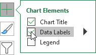
Excel charts: add title, customize chart axis, legend and data labels ... To add a label to one data point, click that data point after selecting the series. Click the Chart Elements button, and select the Data Labels option. For example, this is how we can add labels to one of the data series in our Excel chart: For specific chart types, such as pie chart, you can also choose the labels location.

74 MICROSOFT EXCEL HOW TO CREATE 2D PIE CHART - YouTube

› pie-chart-in-excelPie Chart in Excel | How to Create Pie Chart | Step-by-Step ... In this way, we can present our data in a PIE CHART makes the chart easily readable. Example #2 – 3D Pie Chart in Excel. Now we have seen how to create a 2-D Pie chart. We can create a 3-D version of it as well. For this example, I have taken sales data as an example. I have a sale person name and their respective revenue data.

Creating Pie Chart and Adding/Formatting Data Labels (E... | Doovi

› tutorials › create-pie-chart-inHow to Create a Pie Chart in Google Sheets - Lido Step 3: The selected chart type is not a 3D pie chart by default. On the right side, the Chart editor sidebar is loaded. Click the drop-down box below the Chart type. A list of possible chart types will be loaded. Look for the 3D pie chart, and click it.

How to Create and Format a Pie Chart in Excel

› pie-chart-examplesPie Chart Examples | Types of Pie Charts in Excel ... - EDUCBA It is similar to Pie of the pie chart, but the only difference is that instead of a sub pie chart, a sub bar chart will be created. With this, we have completed all the 2D charts, and now we will create a 3D Pie chart. 4. 3D PIE Chart. A 3D pie chart is similar to PIE, but it has depth in addition to length and breadth.

33 How To Label A Pie Chart In Excel - Labels 2021

Creating Pie Chart and Adding/Formatting Data Labels (Excel) Creating Pie Chart and Adding/Formatting Data Labels (Excel) Creating Pie Chart and Adding/Formatting Data Labels (Excel)

How to Make a Pie Chart in Excel & Add Rich Data Labels to The Chart!

How to Edit Pie Chart in Excel (All Possible Modifications) 7. Change Data Labels Position. Just like the chart title, you can also change the position of data labels in a pie chart. Follow the steps below to do this. 👇. Steps: Firstly, click on the chart area. Following, click on the Chart Elements icon. Subsequently, click on the rightward arrow situated on the right side of the Data Labels option ...

MS Office Suit Expert : MS Excel 2016: How to Create a Pie Chart

Free Pie Chart Maker with Free Templates - Edrawsoft One chart, many forms: EdrawMax doesn't limit you to a circular pie chart; its pie chart maker supports converting your pie chart into a waffle chart, square chart, or 3D forms with a single click. Templates save time & effort.: EdrawMax pie chart maker gives you a quick start to save time and effort with pre-crafted professionally designed templates.

How to Create Excel Pie Charts & Add Rich Data Labels to The Chart!

Display data point labels outside a pie chart in a paginated report ... Create a pie chart and display the data labels. Open the Properties pane. On the design surface, click on the pie itself to display the Category properties in the Properties pane. Expand the CustomAttributes node. A list of attributes for the pie chart is displayed. Set the PieLabelStyle property to Outside. Set the PieLineColor property to Black.

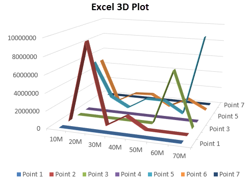
3D Plot in Excel | How to Plot 3D Graphs in Excel?

Add or remove data labels in a chart - Microsoft Support Click the data series or chart. To label one data point, after clicking the series, click that data point. In the upper right corner, next to the chart, click Add Chart Element > Data Labels. To change the location, click the arrow, and choose an option. If you want to show your data label inside a text bubble shape, click Data Callout.

How to Make a Pie Chart in Excel & Add Rich Data Labels to The Chart!

How to Show Percentage in Pie Chart in Excel? - GeeksforGeeks 29/06/2021 · Select a 2-D pie chart from the drop-down. A pie chart will be built. Select -> Insert -> Doughnut or Pie Chart -> 2-D Pie. Initially, the pie chart will not have any data labels in it. To add data labels, select the chart and then click on the “+” button in the top right corner of the pie chart and check the Data Labels button.

Creating a 3D Pie Chart in Excel Vid.wmv - YouTube

Excel 3-D Pie charts - Microsoft Excel 2016 - OfficeToolTips If you want to create a pie chart that shows your company (in this example - Company A) in the greatest positive light: Do the following: 1. Select the data range (in this example, B5:C10 ). 2. On the Insert tab, in the Charts group, choose the Pie button: Choose 3-D Pie. 3. Right-click in the chart area, then select Add Data Labels and click ...

Create a Pie Chart in Excel - Easy Excel Tutorial

r-coder.com › pie-chart-rPIE CHART in R with pie() function [WITH SEVERAL EXAMPLES] An alternative to display percentages on the pie chart is to use the PieChart function of the lessR package, that shows the percentages in the middle of the slices.However, the input of this function has to be a categorical variable (or numeric, if each different value represents a category, as in the example) of a data frame, instead of a numeric vector.

Share :